Angle of Ascent — Dating a Takeoff Photo to the Second
An aerial shot of a KLM Cityhopper lifting off an unnamed runway. Runway markings give the scale, the scale gives the airport, and Denmark's open aerial imagery archive gives a timestamp accurate to the second — enough to name the exact flight and its arrival gate.
The task
This aircraft was captured moments after takeoff. Identify the airport and the plane, then trace its exact flight and determine its arrival gate at its destination.
Flag format:
Hacktoria{ICAO_CALLSIGN_ARRIVAL_GATE}
One image. A light blue airliner over grass, its shadow on the ground beside it, a runway below and a taxiway above. No landmarks, no signage, no horizon. Nothing that a reverse image search will help with.
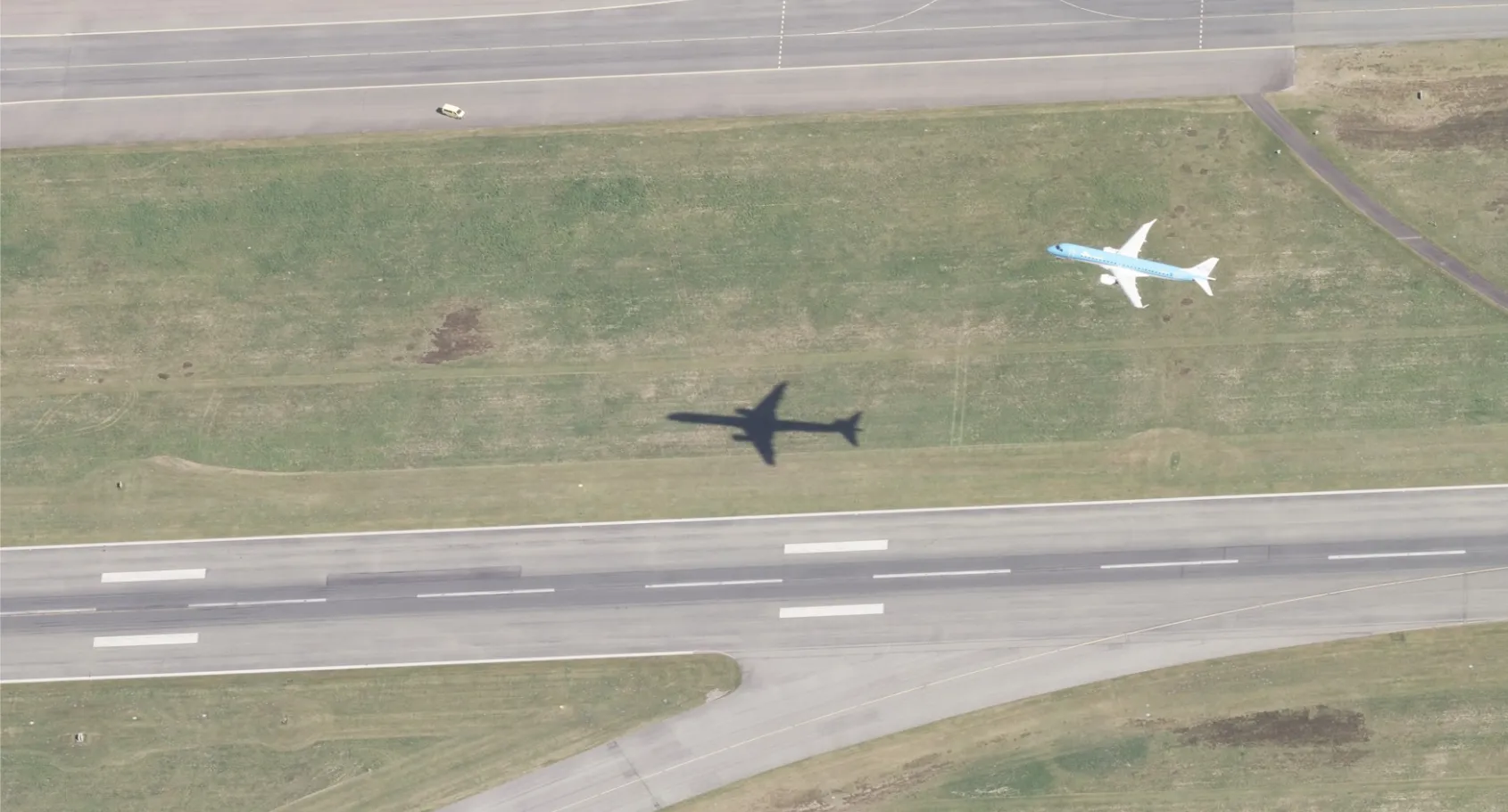
Everything you get: one runway, one parallel taxiway, a wide grass strip, a service vehicle, and an aircraft too small to read a registration off. The shadow ends up mattering twice.
Two things need to come out of this: where and when. The where is a geometry problem. The when turned out to be the interesting part.
The answer, up front: Billund Airport, Denmark — KLM Cityhopper flight KL1292 to Amsterdam, caught mid-rotation by a Danish survey aircraft on 13 May 2025 at 08:24:15 UTC. Callsign KLM46Z, arrival gate B20, flag Hacktoria{KLM46Z_B20}. The rest of this post is how to get there without guessing.
Step 1 — What is the aircraft?
Upscaling the aircraft to 6× answers the first question immediately: the engines are mounted under the wings, not on the rear fuselage. That rules out the Fokker 70/100, which is otherwise the obvious guess for a light blue narrowbody in Northwest Europe.
Light blue fuselage, white wings and tail, regional-jet proportions, wing-mounted engines: KLM Cityhopper, Embraer E-Jet.
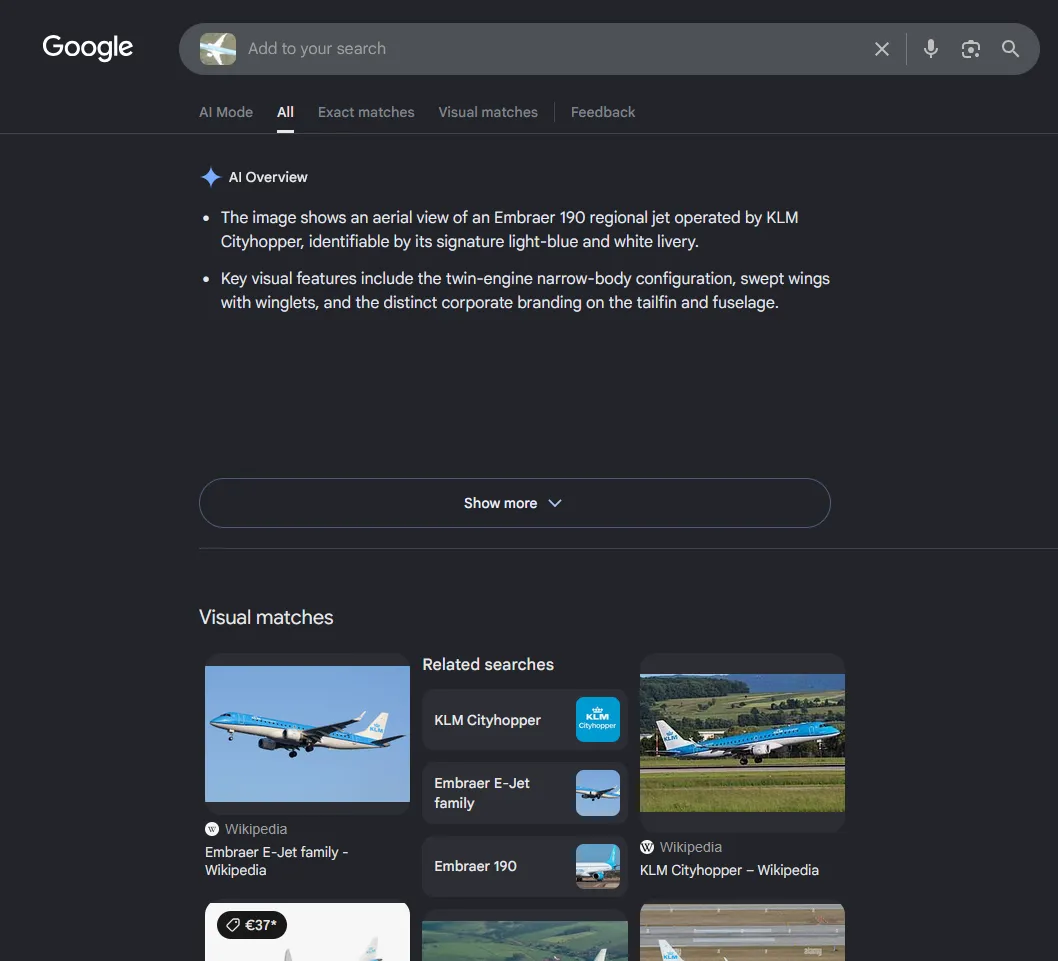
Google Lens on the aircraft crop needs no help — every visual match is a KLM Cityhopper E-Jet. Reverse image search fails on the scene, not on the aircraft.
The registration on the rear fuselage is below the resolution limit. Even with a whiteness-isolation filter (suppressing the blue channel to make white text pop against the light blue paint) it stays unreadable. That’s fine — it isn’t needed.
Step 2 — Narrow the field before measuring anything
The temptation is to start measuring. Resist it — measuring only helps once you have candidates to measure against. Three cheap observations cut the field down first.
The airline gives you a route map. KLM Cityhopper flies short-haul out of Amsterdam. That’s a finite destination list, maybe fifty airports across Northwest Europe.
The imagery type gives you a country group. This is not satellite. The detail is too fine and the perspective is too steep — it’s a survey aircraft. Which means someone flew a mapping mission and, in all likelihood, published it. The countries with genuinely good open aerial imagery portals are a short list: the Netherlands (PDOK), Denmark (Skråfoto), Norway (Norge i bilder), Sweden. That overlaps heavily with the Cityhopper network.
The author gives you a prior. Hacktoria challenges have a Nordic lean (see the note further down). Denmark and Norway first.
The layout gives you a filter. One runway, one parallel taxiway, a wide grass strip between them, no second runway anywhere in frame. Copenhagen is out — two runways. Aalborg and Aarhus don’t match the taxiway geometry. Billund does: a single runway, 09/27, with a parallel taxiway to the north.
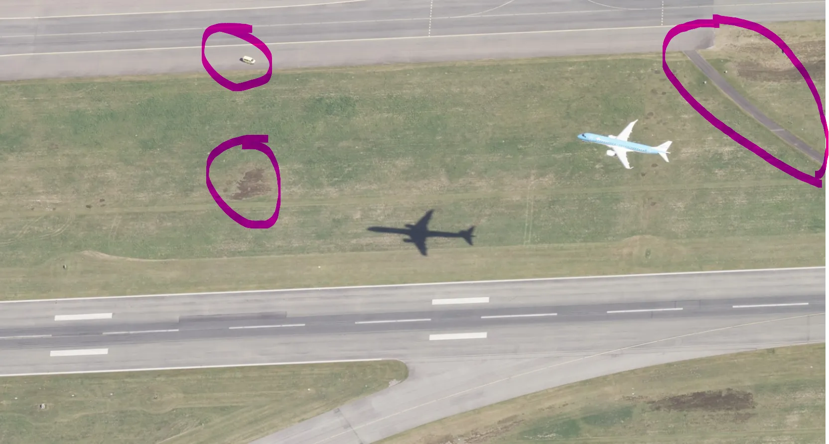
Three anchors picked before any measuring: a vehicle on the taxiway, a bare patch in the grass strip, a dirt track cutting the corner at top right. Whichever airport this is has to show all three in the right places.
That’s ten minutes of work with no arithmetic in it.
Step 3 — Confirm with the runway geometry
Now measuring is worth doing, because there’s a specific claim to test rather than an open-ended search.
The cheap check comes first. Google’s satellite view of Billund shows the same bare patch in the grass and the same dirt track cutting the corner northeast of the taxiway — the anchors from the challenge image, in the same relative positions along runway 09/27.
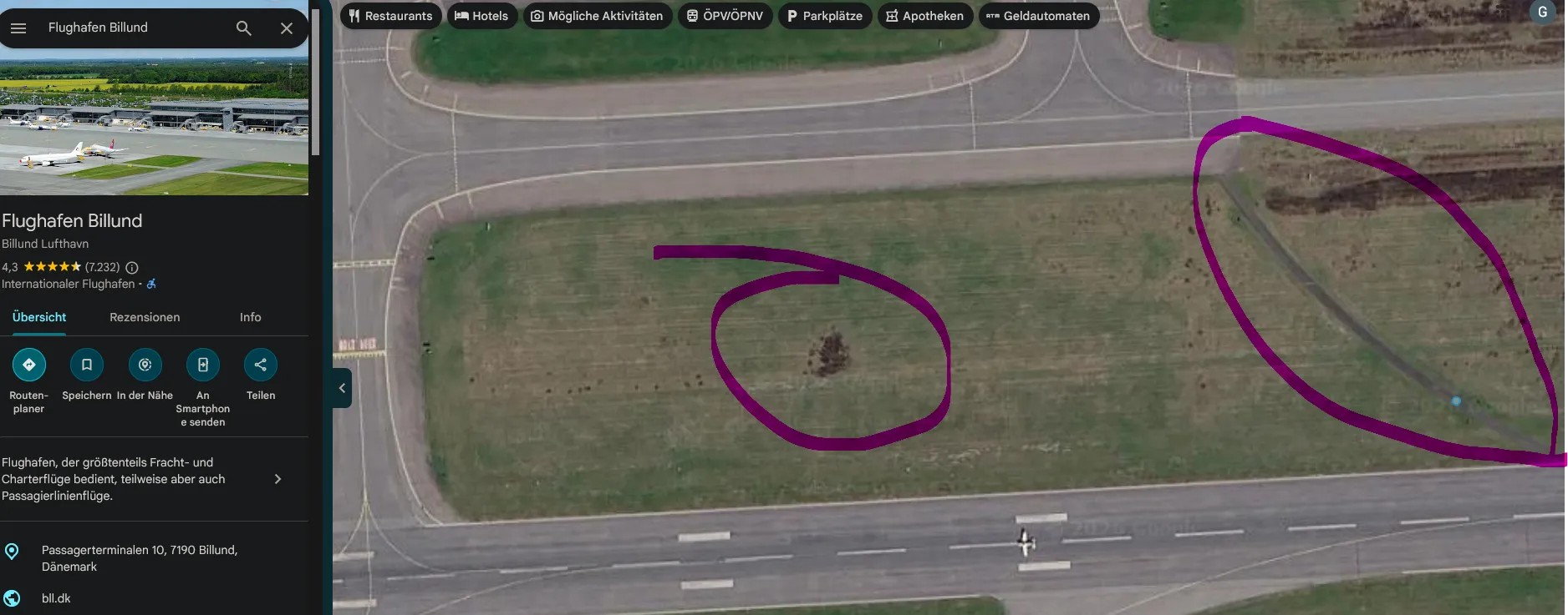
Same patch, same track, same corner — on Google’s imagery of Billund. The layout match is settled before the first measurement; the geometry below is confirmation, not discovery.
Published aerodrome data gives Billund’s runway as 3101 × 45 m. In the image, the distance between the two runway edge lines is 149 px, so if the airport is right, the scale is 45/149 = 0.302 m/px. Everything else in frame should then come out sensible:
| Measurement | In pixels | At 0.302 m/px | Plausible? |
|---|---|---|---|
| Runway edge line to edge line | 149 | 45 m | matches published width |
| Runway CL ↔ taxiway CL | ~574 | ~173 m | standard ICAO Code E separation |
| Image footprint (width) | 1690 | ~510 m | reasonable survey frame |
There’s also a free internal check available. ICAO standardises touchdown zone markings: the bars are 3 m wide with 18 m between their inner edges, putting bar centres at ±10.5 m from the centreline. Measured in the image they sit at ±36 px, which at 0.302 m/px is 10.9 m. Two independent features on the same runway agreeing on the same scale means the scale is right — and by extension the airport is right.
In practice you’d do this with the ruler tool in Google Earth rather than by counting pixels. The point isn’t the precision, it’s that runway markings are standardised worldwide, so any instrument runway in an overhead image is a calibrated ruler you already know the dimensions of.
Step 4 — The timestamp
Here is where this challenge stops being a normal geolocation exercise.
Denmark publishes every aerial photograph of the entire country as open data, with a per-image capture timestamp accurate to the second, through the SDFI/Klimadatastyrelsen service Skråfoto. Four oblique directions (north, south, east, west) plus nadir, roughly every two years since 2017, at about 10 cm GSD.
There is a public web viewer at skraafoto.dataforsyningen.dk, and behind it a STAC API. The API token is not a secret — it sits in the viewer’s own config file at /config.js, which the page loads client-side and which opens with a comment stating that everything in it is public.
Querying every frame that covers a point on the runway:
T=<token from config.js>
curl -s "https://api.dataforsyningen.dk/rest/skraafoto_api/v1.0/search?token=$T" \
  -H 'Content-Type: application/json' -d '{
    "collections":["skraafotos2017","skraafotos2019","skraafotos2021",
                   "skraafotos2023","skraafotos2025"],
    "intersects":{"type":"Point","coordinates":[9.15194,55.74028]},
    "limit":500}' \
| jq -r '.features[] | "\(.properties.datetime) \(.properties.direction) \(.id)"' \
| sort
That returns 104 frames across 10 survey flights, each one a timestamped candidate:
2025-05-13T08:03:47Z west  2025_83_28_5_0009_00006036_100mm
2025-05-13T08:24:11Z north 2025_83_28_2_0008_00006280_100mm
2025-05-13T08:24:15Z north 2025_83_28_2_0008_00006281_100mm
2025-05-13T08:24:19Z north 2025_83_28_2_0008_00006282_100mm
2025-05-13T08:24:35Z nadir 2025_83_28_1_0008_00006286_100mm
...
Each STAC item also carries asset:data, a Cloud-Optimised GeoTIFF that can be windowed directly over HTTP with /vsicurl/ — no need to pull 20544 × 14016 pixels to look at one corner.
Cross-referencing each capture time against the solar position at Billund narrows things considerably, because the shadow in the image encodes the sun elevation. But this is also where I made my first mistake — more on that below.
The aircraft is in the north oblique of the 2025 survey:
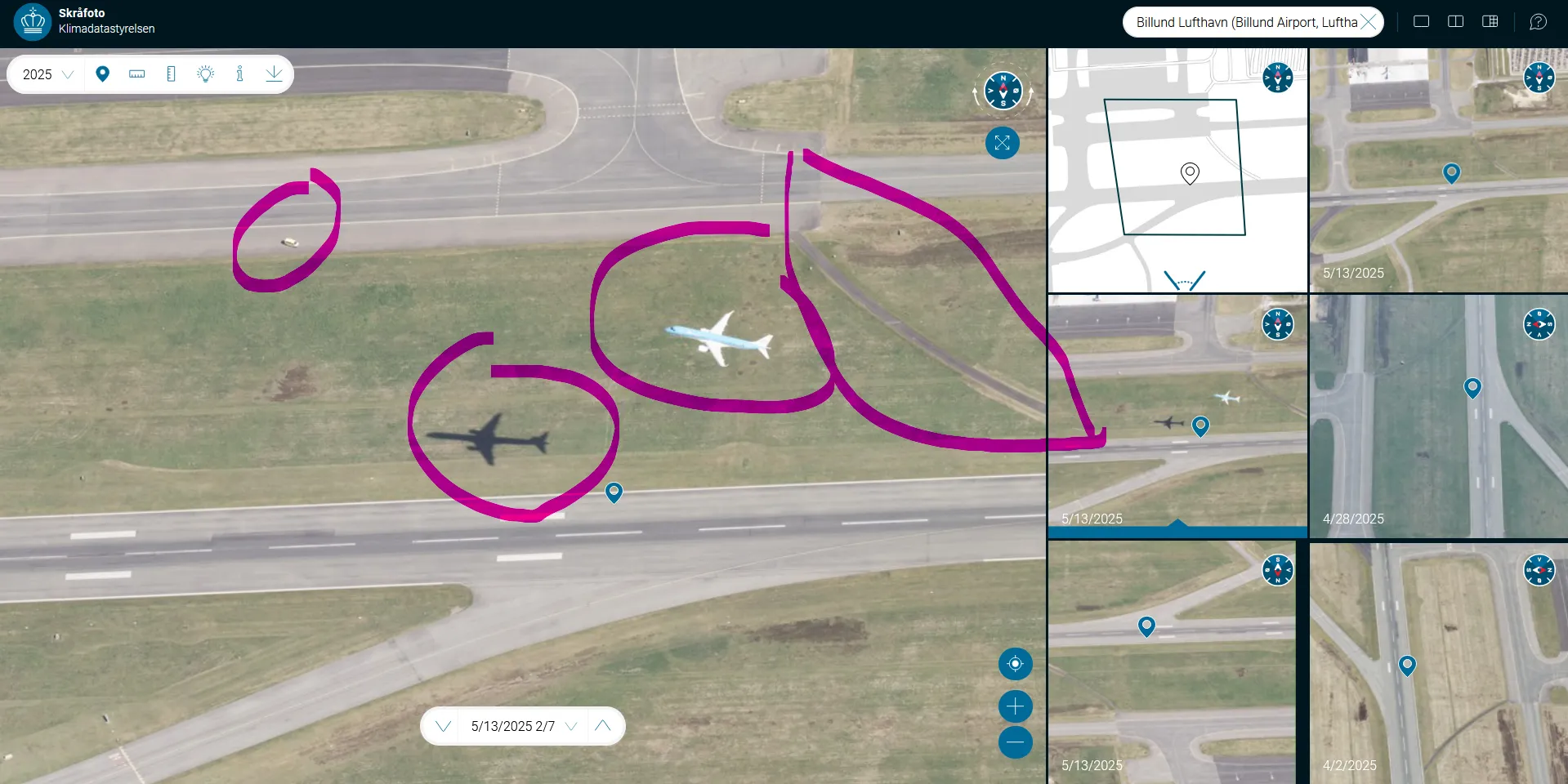
The challenge image, in situ: same aircraft, same shadow, even the same vehicle on the taxiway. Frame 2025_83_28_2_0008_00006281_100mm, north-facing oblique, survey pass 2/7 over Billund.
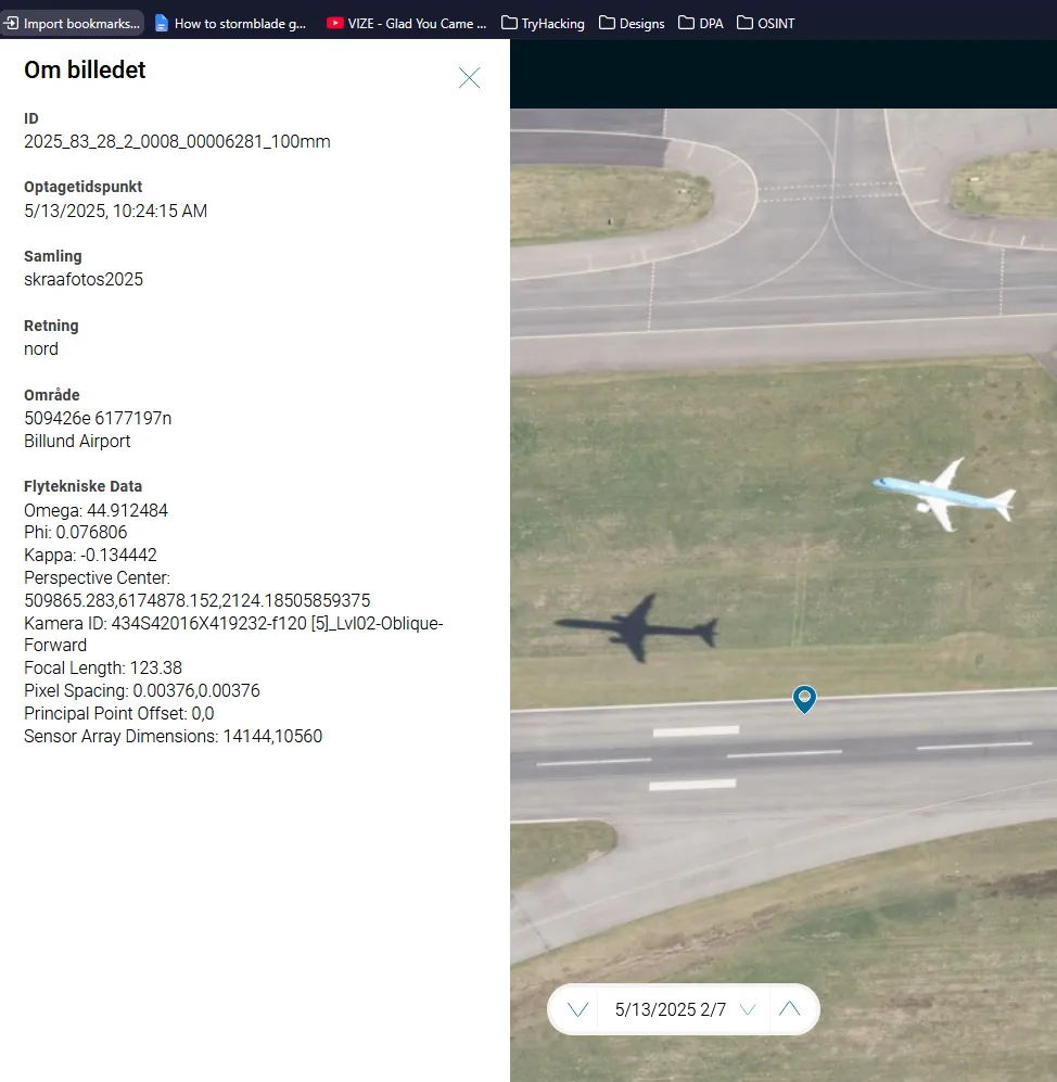
The frame’s own metadata panel: Optagetidspunkt 10:24:15, direction north, collection skraafotos2025 — plus the full camera calibration, down to focal length.
13 May 2025, 10:24:15 local time. Not an estimate. A logged camera trigger.
Step 5 — The flight
Departures from Billund that morning put exactly one KLM service in the window: KL1292 to Amsterdam, scheduled 10:15, operated by KLM Cityhopper on E190/E195 equipment. The livery already fixed the airline, and the timestamp allows only minutes of slack — there is no second candidate to rule out.
Flightera’s history for May 2025 closes it:
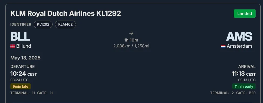
Flightera’s record for 13 May 2025: departure 10:24 CEST, 08:24 UTC, nine minutes late. Everything the flag still needs is in this one header.
The photograph is stamped 08:24:15 UTC. The departure is logged at 08:24 UTC. Same minute. The survey aircraft caught KL1292 in the act of rotating.
The flight detail page supplies the last two fields:
- ICAO callsign: KLM46Z
- Arrival: Amsterdam, Terminal 2, Gate B20
Hacktoria{KLM46Z_B20}Where I went wrong
Two errors, both instructive, both nearly fatal to the solve.
I searched only the nadir frames. My mental model of “aerial survey imagery” was straight-down orthophotos, so that’s what I filtered for. I downloaded and inspected every nadir frame over the airport and found nothing, and briefly concluded the aircraft had been composited into a real photo by the challenge author. It was sitting in an oblique the whole time. When a survey publishes multiple camera directions, search all of them — the interesting frame is often not the one pointing straight down.
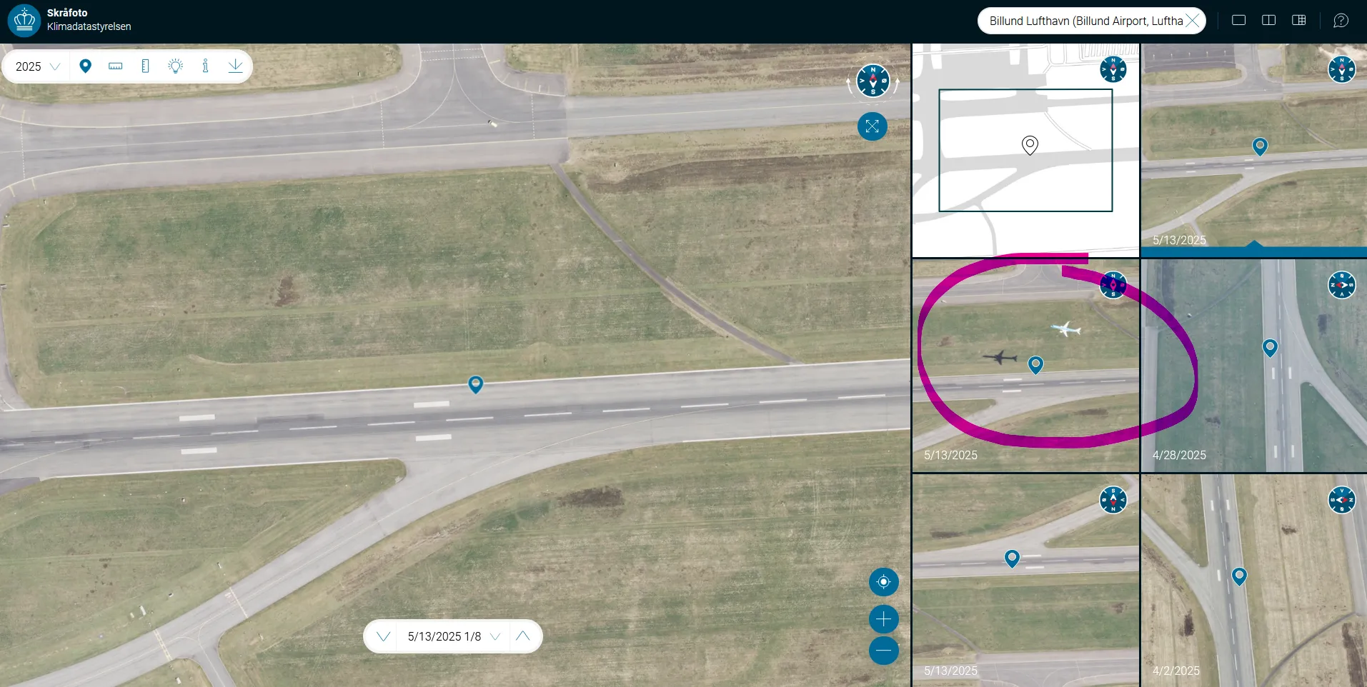
The frame was in the sidebar the whole time — the viewer shows all five directions per date, and the 13 May north thumbnail already contains the aircraft. I was staring at the empty nadir on the left.
I mis-estimated the sun elevation because of that same assumption. Measuring the shadow’s stretch relative to the aircraft gave a factor of about 1.8, implying a sun elevation near 33°. The real value on 13 May at 10:24 is 40°. The error comes from the 45° oblique geometry: the ground is foreshortened along the viewing axis, but an aircraft several hundred metres above that ground is not foreshortened by the same amount. So the aircraft appears roughly 1.5× oversized relative to the terrain, and any shadow-length arithmetic that assumes a common scale comes out wrong.
That discrepancy was actually visible early — the aircraft measured ~58 m long against a scale where an E190 should be 36 m — and I treated it as evidence of compositing rather than as evidence of an oblique view. An anomaly is a clue about the imaging geometry before it’s a clue about tampering.
A note on the author
Worth logging for future Hacktoria challenges: this one lands in Denmark, and an earlier geolocation challenge put me in Norway (a farmhouse brewery, Rodebak Gårdsbryggeri). That’s a small sample, but the Nordic lean is there.
It’s a soft prior, not a shortcut — never let it override what the image actually shows. But it has practical value in how you order your work. When an image gives you a shape to match and no name, the question is which candidate list to walk first, and starting with Scandinavia would have saved me a pass here. It also pays off downstream: Denmark, Norway, Sweden and Finland all run national open geodata programmes with far better aerial coverage and metadata than most of Europe. If the challenge is set in the Nordics, the odds are good that a timestamped orthophoto or oblique exists for the exact scene, which is precisely what carried this solve.
So: keep a running note on where a given author sets their challenges. It won’t identify anything on its own, but it tells you which archives to have open before you start.
Takeaways
Runway markings are a calibrated ruler — but use them to confirm, not to search. ICAO standardises edge line placement, centreline dimensions, touchdown zone bars and aiming point markings, so any overhead image of any instrument runway carries a known scale. What that gets you is verification: once you have a candidate airport, two independent measurements agreeing on one scale settles it. What it does not get you is the candidate. Narrow the field with cheap observations first — airline, imagery source, layout, author habits — then measure.
Denmark timestamps its aerial imagery to the second, and gives it away. For any GEOINT task on Danish soil, Skråfoto is not a nice-to-have — it converts “roughly what year” into “which second”. Combined with ADS-B history, that’s enough to identify individual aircraft movements. Similar national orthophoto programmes exist elsewhere (the Netherlands’ PDOK, Norway’s Norge i bilder), though not all expose per-frame capture times as cleanly — the technique page on open aerial archives collects the portals and the query workflow.
API tokens in client-side config are public by design. The Skråfoto viewer’s config file says so explicitly in a comment. Reading the front end of a public map viewer to find its data endpoint is standard practice, not a bypass.
Sources
- Skråfoto viewer — Klimadatastyrelsen’s oblique aerial imagery archive; the STAC API behind it is at
api.dataforsyningen.dk/rest/skraafoto_api/v1.0 - Dataforsyningen documentation — API reference for the Skråfoto STAC endpoints
- Billund Airport — Wikipedia — runway 09/27, 3101 × 45 m
- FAA AIM — Airport Marking Aids and Signs — standard dimensions for edge lines and touchdown zone bars (mirrors ICAO Annex 14)
- KLM Cityhopper — Wikipedia — fleet and route network
- Flightera — KL1292 flight history for 13 May 2025, including callsign and arrival gate
- SunCalc — solar elevation at Billund for the shadow cross-check
- Hacktoria — the Angle of Ascent challenge
Image credits
Aerial imagery (challenge image, annotated crops, cover, and viewer screenshots):
Skråfoto oblique photograph 2025_83_28_2_0008_00006281_100mm and surrounding
frames © Klimadatastyrelsen (Danish
Climate Data Agency), licensed under
CC BY 4.0.
Modified: cropped, resized, and annotated for analysis.
Layout-verification screenshot: map data © Google. Google Lens and Flightera
screenshots reproduced for the purpose of analysis and commentary.